July 2022
Neural networks are often treated as black boxes that give results without telling how and why. Various methods have been proposed to explain their decisions over the last decade. Here, we present a method, recently published in ECCV 2022, which finds the relevant piece-wise smooth part of an image for a neural network decision using wavelets.
Neural networks are powerful function approximators that can be trained on data to solve complex tasks, such as image classification. However, the expressive power of neural networks comes with a price: Neural networks are not inherently interpretable. It’s difficult to say why a network \(f_\theta\) decides to assign an image \(x\) the label \(y=f_\theta({\color{orange}x})\), let alone to say what constitutes a good model explanation. Over the last decade, research yielded many competing approaches to these questions. One popular and particularly intuitive framework is the mask-based explanation framework. The idea is quite simple: a good explanation for \(y=f_\theta({\color{orange}x})\) is a mask \(m\in\{0,1\}^d\) over the input \({\color{orange}x}\in\mathbb{R}^d\) that masks the irrelevant input features. The mask captures the relevant components in \({\color{orange}x}\) if they determine the model output. To test that, we require that for all meaningful perturbations \(\xi\in\mathbb{R}^d\) the so-called distortion is small:
\[\begin{aligned} \label{eq: model output diff} \|f_\theta({\color{orange}\underbrace{x}_{\text{input}}}) - f_\theta({\color{Blue}\underbrace{m \odot x + (1-m)\odot \xi}_{\text{perturbed input}}}) \|_2\approx 0.\end{aligned}\]
But what exactly constitutes a meaningful perturbation? We typically assume that data lies on a low-dimensional manifold. Ideally, replacing the masked parts of the image with our perturbation should keep the result \(\color{Blue} m \odot x + (1-m)\odot \xi\) in the manifold of the underlying data distribution for the classification task of \(f_\theta\). This would ensure that \(f_\theta\) still behaves well on the new input. In practice, modeling the conditional input distribution may be difficult or infeasible. In that case, we can resort to heuristic choices such as Gaussian noise perturbations, inpainting with another neural network, or infilling with an constant average.
Below, you can draw some masks yourself. Then press the button "Predict with Neural Network" to calculate the expected distortion and the most likely classification for a small neural net called MobileNet after perturbing unselected pixels with Gaussian noise. Can you guess which parts of the images are important for the MobileNet?
Original
Mask (draw here!)
Perturbed Image
Average Distortion:
Top label:
Of course, we don't want to guess and draw multiple masks ourselves in practice to explain a neural net. Instead we want an algorithm that finds a good explanation mask efficiently.
How can we find a "good" explanation mask? It turns out, all we need to do is solve an optimization problem. First, we model perturbations as a random variable \(\xi \sim \Xi\), where \(\Xi\) is a pre-chosen probability distribution (e.g. Gaussian). We say a sparse mask \(m\in\{0,1\}^d\) is a good explanation mask for \(x\) if the model output for \({\color{orange}x}\) is on average approximately the same as for the masked and perturbed input \(\color{Blue} m \odot x + (1-m)\odot \xi\). Formally, this condition is
\[\begin{aligned} \label{eq: expected model output diff} {\color{black}\mathop{\mathbb{E}}_{\xi\sim\Xi}\Big[\|f_\theta({\color{orange}x}) - f_\theta({\color{Blue}m \odot x + (1-m)\odot \xi}) \|_2\Big]\approx 0.}\end{aligned}\]
Note that the trivial mask \(m = \begin{bmatrix}1 & \dots & 1 \end{bmatrix}^T\) always satisfies this condition with strict equality. However, that mask does not provide any explanatory information because it does not tell us which features are not relevant for the classification decision. To find useful and concise explanatory information about \(f_\theta({\color{orange}x})\), we need to find a sparse mask \({m}\) satisfying the condition above. Finding the explanation mask \(m\) becomes an optimization problem:
\[\begin{aligned} \label{opt: explanation mask} \min_{{m}\in\{0,1\}^d} \mathop{\mathbb{E}}_{\xi\sim\Xi}\Big[\|f_\theta({\color{orange}x}) - f_\theta({\color{Blue}m \odot x + (1-m)\odot \xi}) \|_2\Big] \;\;\;\;\;\; \textrm{s.t.}\;\; \|{m}\|_0 = l,\end{aligned}\]
where \(0<l<d\) is a pre-specified desired sparsity level. Most interesting applications involve high-dimensional inputs \({\color{orange}x}\in\mathbb{R}^d\) (e.g. for images \(d\) is in the order of the number of pixels) and solving the optimization problem becomes computationally infeasible. Still, we can try to approximately solve it by solving the Lagrangian relaxation
\[\begin{aligned} \label{opt: lagrangian relaxation} \min_{{m}\in[0,1]^d} \mathop{\mathbb{E}}_{\xi\sim\Xi}\Big[\|f_\theta({\color{orange}x}) - f_\theta({\color{Blue}m \odot x + (1-m)\odot \xi}) \|_2\Big] + \lambda \|{m}\|_1,\end{aligned}\]
where \(\lambda>0\) determines the sparsity level of the relaxed continuous mask \(m\in[0,1]^d\). Although the mask \(m\) is no longer binary in the relaxed optimization problem, the \(\ell_1\)-term promotes sparsity and produces useful explanatory insight in practice. In practice, the expectation can be approximated with a simple Monte-Carlo estimate and the relaxed optimization problem can be solved with gradient descent over the input mask \(m\).
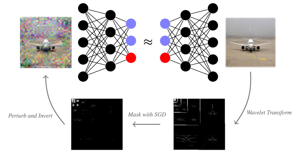
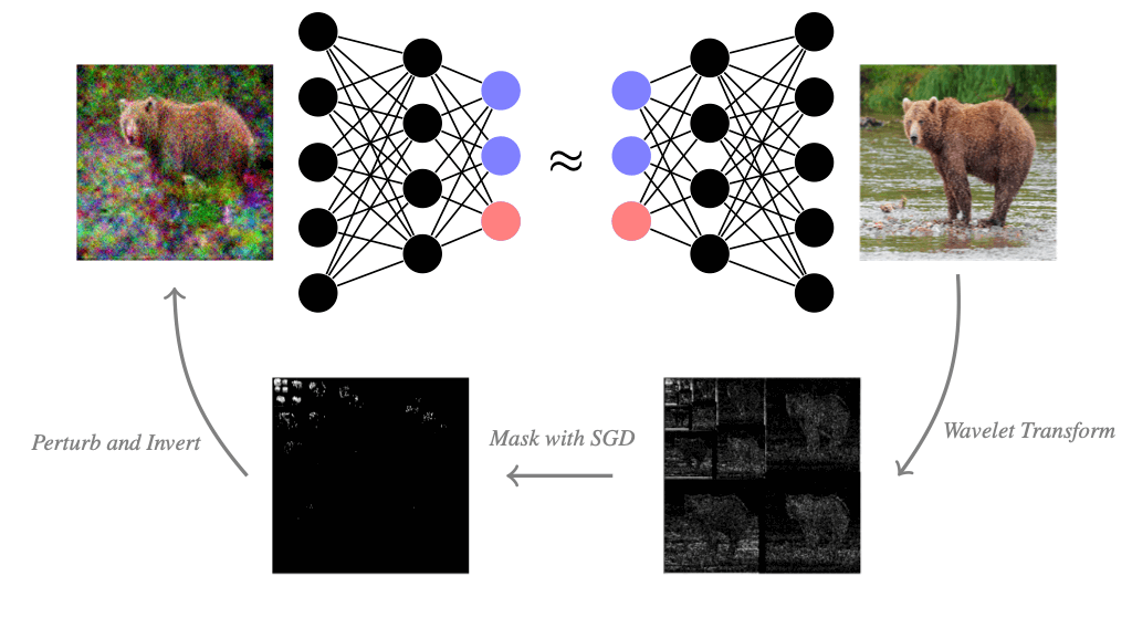
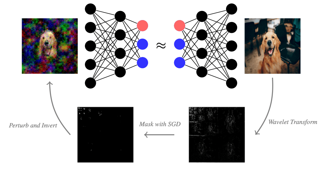
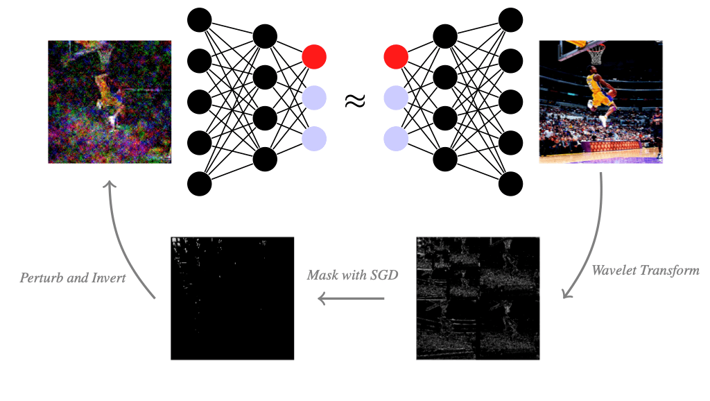
How can we apply the above framework to images? Images are typically represented as an array of shape \(\mathbb{R}^{n\times m\times c}\), where the image has a resolution of \(n\times m\) pixels and \(c\) different color channels per pixel. If we apply the mask-based explanation method to images in the pixel basis, then we would get the most important color channels of all pixels. But that is not particularly meaningful for us humans. We could also mask all colors of pixels at once and explain pixel-wise, which is a common approach for explaining image classifiers. Then the masking method would give us the most important pixels. However, we usually don't care about single pixels and a set of pixels can potentially look very jittery. We would instead like to find relevant piece-wise smooth image regions. This is where the so-called wavelet transform can help us. By applying the wavelet transformation, we still represent the images as an array of numbers, but instead of the brightness of a single pixel, each number can represent a larger structure. The wavelet transform tends to be not as widely known as the Fourier transform outside the signal processing community. Therefore, we will briefly explain the wavelet transform, which is an essential tool in signal processing and has plenty of applications beyond explainability in data science and machine learning.
Scale
Position
Mother wavelet
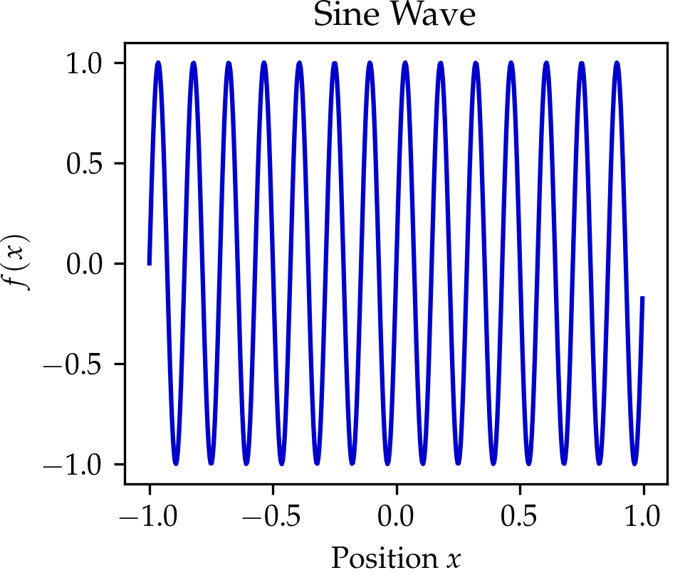
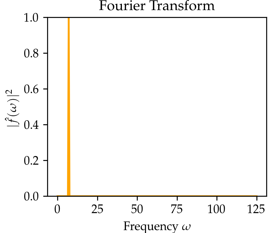
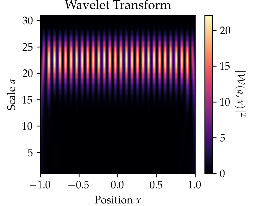
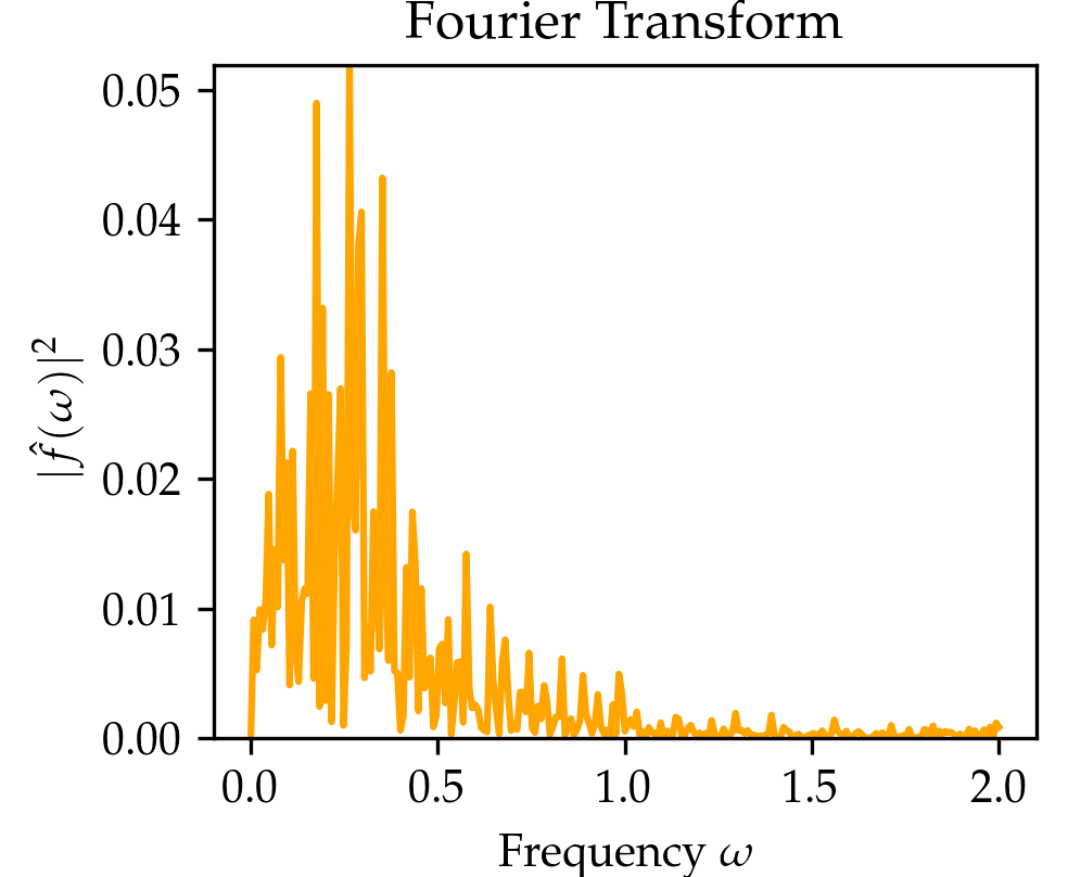
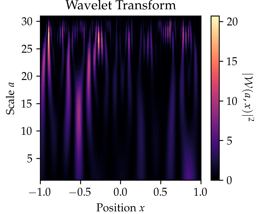
The wavelet transform is very closely related to the well-known Fourier transform. The Fourier transform convolves a signal \(x\mapsto f(x)\) with sinusoids \(x\mapsto e^{-i2\pi\xi x }\) of different frequencies \(\xi\), thereby decomposing the signal \(x\mapsto f(x)\) into their frequency components \(f(\xi)\) through the relationship \[\hat f(\xi) \coloneqq \int_{-\infty}^{\infty}e^{-i2\pi\xi x}f(x)\,dx.\] The Fourier Transform has full frequency resolution but no spatial resolution, meaning we can say which frequencies \(\xi\) occur in the signal \(x\mapsto f(x)\) but not at what position \(x\). The wavelet transform extracts both spatial and frequency information by convolving a signal \(x\mapsto f(x)\) not with sinusoids but so-called wavelets (denoted as \(x\mapsto \psi(x)\) and referring to a wave-like oscillation), which are localized in space to provide additional spatial information unlike the sinusoids. The wavelet transform filters a signal (e.g. an image) with a filter \[\begin{aligned} x\mapsto \frac{1}{\sqrt{a}}\psi\Big(\frac{x-b}{a}\Big) \end{aligned}\] that is localized in frequency (represented by a scale parameter \(a\)) and position (represented by parameter \(b\)). In practice, there are many possible wavelets \(\psi\) to choose from, such as Haar or Daubechies wavelets.
| Transform | Formula | Parameters |
|---|---|---|
| Fourier Transform | \(\hat f(\xi) \coloneqq \int_{-\infty}^{\infty}e^{i2\pi\xi t}f(t)\,dt\) | Frequency \(\xi\) |
| Wavelet Transform | \(\mathcal{W}f(a, b) \coloneqq \frac{1}{\sqrt{a}}\int_{-\infty}^\infty \psi\Big(\frac{t - b}{a}\Big)f(t)\,dt\) | Scale \(a\), Position \(b\), Mother wavelet \(\psi\) |
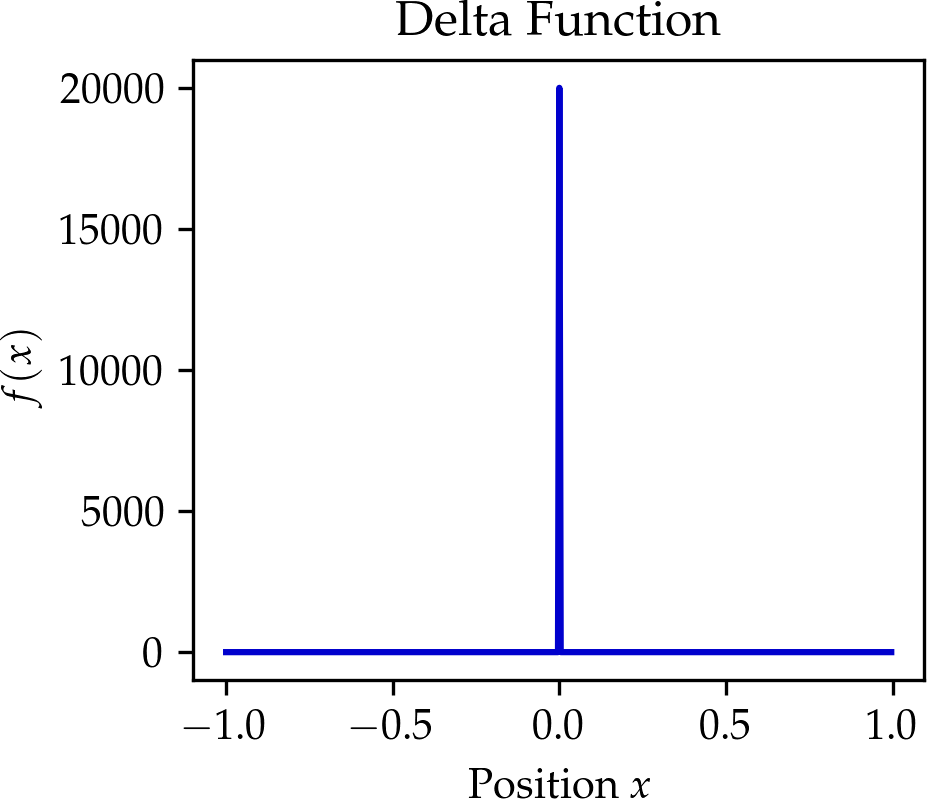
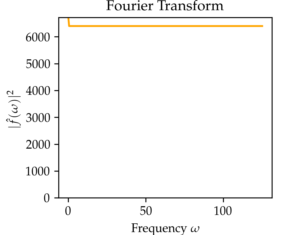
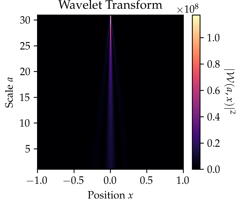
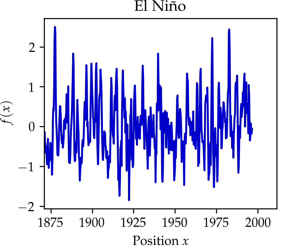
We compare the wavelet transform to the Fourier transform in the Table above and the figure below. In the figure below click on the button to select beween three signals. You might notice that the wavelet transform can localize the sine oscillations and the delta function peak, as well as give time-frequency information for the signal in the El Niño dataset (quarterly measurements of the sea surface temperature from 1871 up to 1997 throughout the equatorial Pacific).
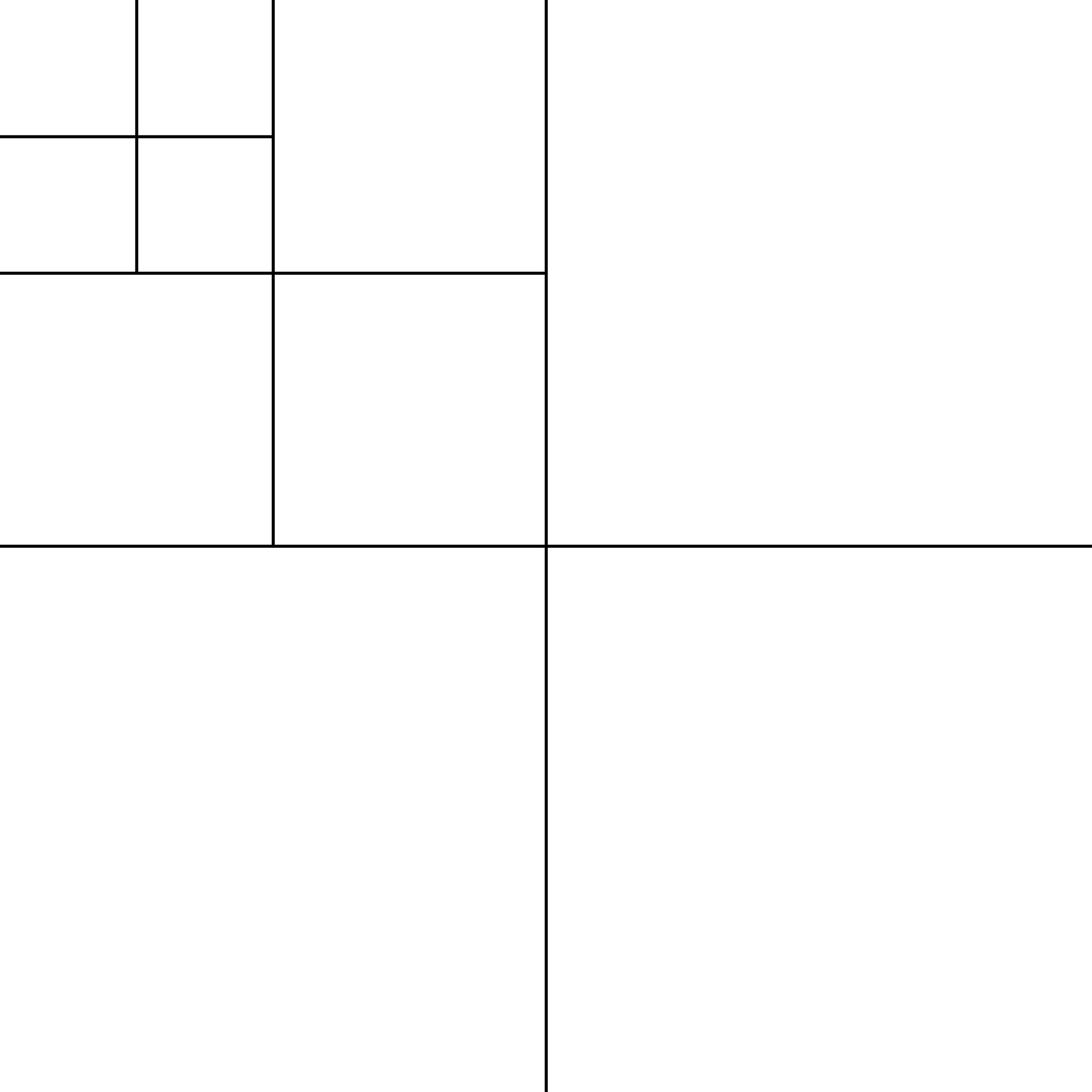
Now that we understand the wavelet transform in one dimension, we can go back to images, which are two-dimensional signals. Just like the Fourier transform, the wavelet transform can be extended to two dimensions. Since images are discrete objects, we use the discrete wavelet transform, which works similarly to the discrete Fourier transform. You can draw in the box below to get a live visualization of the two-dimensional discrete wavelet transform for the Haar wavelet. Roughly speaking, a single Haar wavelet can represent a square. With that, it can fairly accurately represent images with fewer non-zero numbers. If you draw on the left side below, it will automatically calculate the Haar wavelet transform of the drawn image and represent its wavelet coefficients on the right side. Each quadrant represents a wavelet coefficient \(\mathcal{W}(a,b)\) at a scale \(a\) and pixel position \(b.\) The small scales correspond to large quadrants and fine details features. For each scale \(a\), there are three quadrants representing horizontal, vertical, and diagonal wavelet filtering. Try drawing a larger region, and you will see that most of the image on the right remains blank. This is because natural images tend to be sparse in the wavelet domain (few non-zero wavelet coefficients), a property which is also used by image compression algorithms.
Pixel image
Discrete wavelet transform
Now that we are familiar with wavelets, let’s go back to explaining neural nets. We can also generate a mask-based explanation in the wavelet basis by optimizing a mask on the wavelet coefficients of an image. When we mask wavelet coefficients, we keep a piece-wise smooth image because wavelets sparsely represent piece-wise smooth images well. After masking wavelet coefficients, we can visualize the wavelet mask in pixel space by applying the inverse wavelet transform to the wavelet coefficients. The result is a piece-wise smooth image that suffices to keep the classification decision. Irrelevant image regions are blurred or black, and fine details that are kept are relevant to the classifier. To contrast the explanation from the original image, we visualize the wavelet-based explanation in grayscale. When we mask in the wavelet basis, we still have to choose the sparsity parameter \(\lambda\), which controls how many coefficients are masked. Larger \(\lambda\) will mask more wavelet coefficients and thus blur or black out more of the image. A good \(\lambda\) deletes not too little and not too much information in the image. We found that wavelet-based explanations can convey interesting explanatory insight and are often visually more appealing than their jittery pixel-mask counterparts. Try it yourself and play around below by choosing an image and the sparsity parameter \(\lambda\) for the mask.
Original

Wavelet Mask
Pixel Mask
Wavelets are established tools in signal processing and have found various applications in data science and machine learning. More recently, wavelets were also used to explain neural network decisions, generating novel piece-wise smooth wavelet-based explanations that are particularly suitable for image classifiers. We think wavelet-based explanations will be a useful addition to the practitioners’ explainability toolbox and inspire researchers to further improve explanation methods.
For a more complete explanation, see the original paper.
We thank Ron Levie, Manjot Singh, Chirag Varun Shukla, and other members of the Bavarian AI Chair for Mathematical Foundations of Artificial Intelligence for their support and feedback.
This article and the widgets are licensed under Creative Commons Attribution CC-BY 4.0. Image credits: Black swan, zebra, kangaroo, leopard, scorpion, lighthouse, airplane, elephant, dalmatian, deer, fox, bear.
.jpg)
.jpg)